Here, we’ll take a detailed look at overfitting, which is
one of the core concepts of machine learning and directly related to the suitability of a model to the problem at hand. Although overfitting itself is relatively straightforward and has a concise
definition, a discussion of the topic will lead us into a range of related fields such as model regularization and learning curves, which are tools to assess model suitability.
Recall that in all machine learning applications we are
trying to learn about some non-obvious structure in the data. In the case of supervised learning, this involves the creation of some hypothesis function, which we hope is as close a fit as
possible to the true relationship between the features and the target. The complexity of the hypothesis function will vary depending on the algorithm we choose and the hyperparameters it
uses.
This leads us to the question, how complex should our
hypothesis function be? How do we know when it is too complex or not complex enough?
Some algorithms (e.g. neural networks, gradient boosted trees etc.) are capable of producing
very complicated hypothesis functions. This is great if such a hypothesis function is warranted by the data, but may produce poor results if not. The topic of overfitting is intricately linked to
algorithm choice, and serves as a reminder that the most suitable algorithm for a problem is often not the most complicated or most advanced.
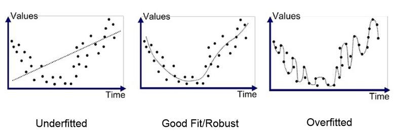
At this point, lets define overfitting and under-fitting in
the context of the hypothesis function
-
Overfitting: When the statistical model
contains more parameters than justified by the data. This means that it will tend to fit noise in the data and so may not generalize well to new examples. The hypothesis function is too
complex.
-
Underfitting: When the statistical
model cannot adequately capture the structure of the underlying data. The hypothesis function is too simple
In machine learning practice, there is a standard way of
trying to avoid these issues before a model is deployed. This involves spitting the available dataset into train, test and holdout sets, typically with something like a 60%, 20%, 20%
split.
The model is allowed to learn from the training dataset and
its performance is assessed on that dataset to provide a ‘training score’. Ideally the training score should be high because the model has
been allowed to see all of the data that it is subsequently being scored on.
The model is then applied to the test dataset and a
‘testing score’ obtained. This should generally be lower than the
‘training score’ since the model has never seen the testing data and so has not
been able to learn any additional structure that wasn’t present in the training dataset. Usually the model can be improved by variation of hyperparameters, retraining and then retesting,
typically using a method like k-fold cross validation, which we will address in a future post.
Once the training score has been maximized, the final model
is applied to the holdout dataset, which is a completely unseen set of data that will provide the best sense of how the model will perform in the real world. ''
If a model is overfitting, it will generally perform well
very the training set because it is sufficiently complex to start fitting noise in the data. However, it will perform poorly on the test (and holdout) data because it overcomplicates the true structure of the data
and so is unable to generalize.'
In the case of underfitting, performance on both the
training and testing datasets will be poor because the model is unable to capture the complexities of the dataset.
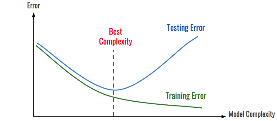
A graph of training and testing error vs model complexity
provides a good illustration of the tradeoff between underfitting and overfitting. The best model is the one the provides a hypothesis function that is closest to the true relationship within the
data. Such a model will produce a minimum in testing error. To the left of this minimum, simpler models will be underfitting. To the right, more complex models will be overfitting.
What do we actually mean by model complexity? This can be related to a great many things and so is difficult to quantify. It is related to the hyperparameter choices for the algorithm - such as
the size of the regularization term in linear regression, the maximum tree depth for decision trees, the number of layers in a neural network etc. These are usually things that can be optimized
during testing. However, model complexity is also related to the number of features and the size of the dataset. Typically the more features are used, the more complex the model becomes.
Another concept, which will add provide insight into
relationship between overfitting and model complexity, is the bias-variance decomposition of error, also known as the bias-variance tradeoff
-
Bias is the contribution to total error
from the simplifying assumptions built into the method we chose
-
Variance is the contribution to the
total error due to sensitivity to noise in the data. For example, a model with high variance is likely to produce quite different hypothesis functions given different training sets with the
same underlying structure just due to different noise in two datasets.
The bias-variance tradeoff refers to the fact that models
with high bias will have low variance and vice versa, so it it important to choose a model that has an optimal contribution from both such that total error is minimized
As clearly shown in the graph above, models with high bias
tend to under-fit, while models with high variance tend to overfit. This makes intuitive sense given the definitions of overfitting and underfitting.
How can we turn knowledge about underfitting or overfitting
into actionable insights that can be applied to improve the model? One of easiest ways of doing this is to plot learning curves.
To generate a learning curve, we need to artificially reduce
the size of the testing dataset in a series of steps. At each step, we train a model (using the same hyperparameters each time) and then report the training and
testing errors (or the training and testing scores for classification problems). When the
training dataset is small, the model should be able to fit very well (it will overfit), but will not generalize to the testing or holdout sets.
When the training dataset is larger, the training error should be larger, but the testing error should reduce.
The shape and similarity of the training and testing error
curves as a function of training set size will potentially inform us about whether the model has a bias or variance problem and give clues about what to do about it.
If the model has a bias problem (underfitting), then both the testing and training error curves will plateau quickly and
remain high. This implies that getting more data will not help! We can improve model performance by reducing regularization and/or by using an algorithm capable of learning more complex
hypothesis functions.
If the model has a variance problem (overfitting), the training error curve will remain well below the testing error and
may not plateau. If the training curve does not plateau, this suggests that collecting more data will improve model performance. To prevent overfitting and bring the curves closer to one
another, one should increase the severity of regularization, reduce the number of features and/or use an algorithm that can only fit simpler hypothesis functions.